Part 2: Integrating Parkinson’s disease cohorts

Part 2: Integrating Parkinson’s disease cohorts#

This notebook is a continuation of demoing the utility of mgnipy in curating cross-study datasets from MGnify for secondary analysis.

Here we further preprocess the curated dataset we obtained from Part 1. Specifically we preprocess the count data and then use ABaCo for batch/technical variance correction, following their PD demo

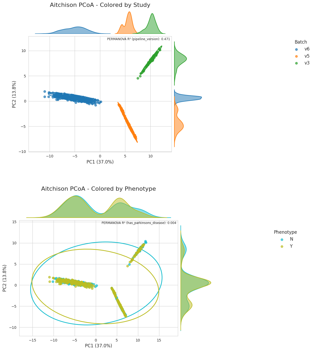
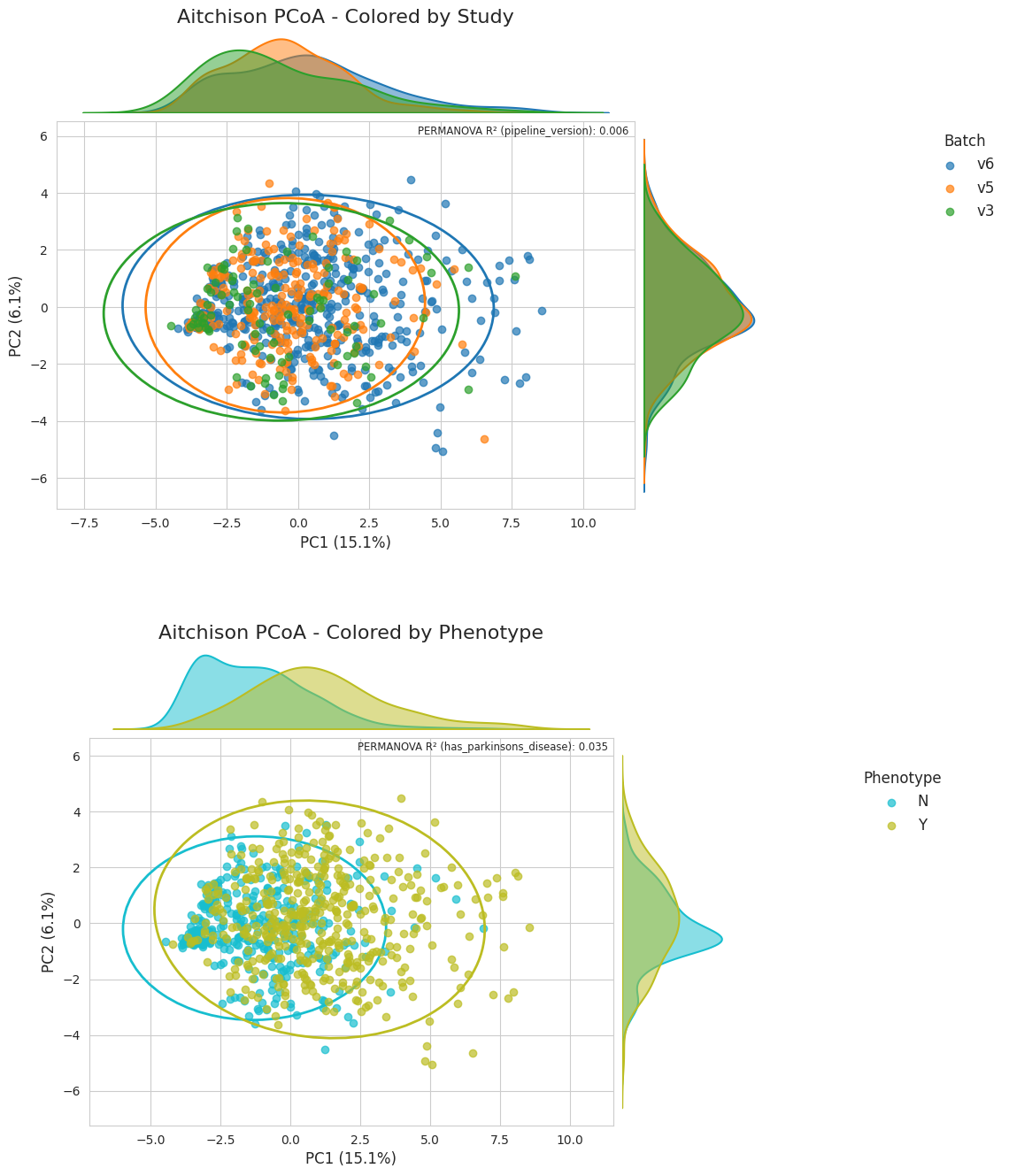
Using abaco we aim to mitigate the technical variance across the 6 MGnify studies.

# uncomment if colab
# !pip install abaco

Loading the dataset from Part 1#

import anndata as ad
import httpx
from io import BytesIO

url = "https://github.com/EBI-Metagenomics/mgnipy/raw/refs/heads/tidyup-demos/docs/notebooks/demos/pd.h5ad"
r = httpx.get(url, follow_redirects=True)
r.raise_for_status()

# read in
ad_tax = ad.read_h5ad(
    BytesIO(r.content)#'pd.h5ad'
)
# check it out
ad_tax

AnnData object with n_obs × n_vars = 1606 × 3247
    obs: 'experiment_type', 'instrument_model', 'instrument_platform', 'sample_accession', 'study_accession', 'updated_at', 'run_accession', 'status', 'pipeline_version', 'sample__accession', 'sample__ena_accessions', 'sample__sample_title', 'sample__biome', 'sample__updated_at', 'study__accession', 'study__ena_accessions', 'study__title', 'study__updated_at', 'study__biome.biome_name', 'study__biome.lineage', 'study__metadata.study_name', 'study__metadata.center_name', 'study__metadata.study_title', 'study__metadata.study_accession', 'study__metadata.study_description', 'study__metadata.secondary_study_accession', 'GivenID', 'RunID', 'SRA accession', 'name', 'taxid', 'ENA first public', 'ENA-CHECKLIST', 'External Id', 'INSDC center name', 'INSDC last update', 'INSDC status', 'Submitter Id', 'broad-scale environmental context', 'collection date', 'description', 'environmental medium', 'geographic location (country and/or sea)', 'geographic location (latitude)', 'geographic location (longitude)', 'host age', 'host diet', 'host disease status', 'host family relationship', 'host sex', 'host subject id', 'local environmental context', 'organism', 'project name', 'scientific_name', 'sequencing method', 'title', 'ENA-FIRST-PUBLIC', 'ENA-LAST-UPDATE', 'INSDC first public', 'age', 'body product', 'disease status', 'environment (biome)', 'environment (feature)', 'environment (material)', 'geographic location (countryand/orsea,region)', 'human gut environmental package', 'investigation type', 'medical history performed', 'miscellaneous parameter', 'multiplex identifiers', 'pcr primers', 'sex', 'target gene', 'target subfragment', 'host body product', 'parkinson', 'timepoint', 'sample collection device or method', 'sample storage duration', 'sample storage temperature', 'gastrointestinal tract disorder', 'INSDC secondary accession', 'NCBI submission model', 'NCBI submission package', 'env_broad_scale', 'env_local_scale', 'env_medium', 'geo loc name', 'host', 'host_phenotype', 'isolate', 'status__biosamples_metadata', 'isolation source', 'lat lon', 'collection_date', 'descrip', 'geo_loc_name', 'isolation_source', 'lat_lon', 'Age_at_collection', 'Anti_inflammatory_drugs', 'Antibiotics_current', 'Antibiotics_past_3_months', 'Antihistamines', 'Asthma_or_COPD_med', 'BMI', 'BioSampleModel', 'Birth_control_or_estrogen', 'Blood_pressure_med', 'Blood_thinners', 'Bristol_stool_chart', 'Case_status', 'Celiac_disease', 'Cholesterol_med', 'Co_Q_10', 'Colitis', 'Constipation', 'Crohns_disease', 'Day_of_stool_collection_abdominal_pain', 'Day_of_stool_collection_bloating', 'Day_of_stool_collection_diarrhea', 'Day_of_stool_collection_excess_gas', 'Depression_anxiety_mood_med', 'Diabetes_med', 'Diarrhea', 'Do_you_drink_alcohol', 'Do_you_drink_caffeinated_beverages', 'Do_you_smoke', 'GI_cancer_past_3_months', 'Gained_10lbs_in_last_year', 'Hispanic_or_Latino', 'How_often_do_you_eat_FRUITS_or_VEGETABLES', 'How_often_do_you_eat_GRAINS', 'How_often_do_you_eat_NUTS', 'How_often_do_you_eat_POULTRY_BEEF_PORK_SEAFOOD_EGGS', 'How_often_do_you_eat_YOGURT', 'IBD', 'IBS', 'INSDC center alias', 'Indigestion_drugs', 'Intestinal_disease', 'Jewish_ancestry', 'Laxatives', 'Loss_10lbs_in_last_year', 'Pain_med', 'Probiotic', 'Race', 'Radiation_Chemo', 'SIBO', 'Sex', 'Sleep_aid', 'Thyroid_med', 'Ulcer_past_3_months', 'broker name', 'collection_method', 'Day_of_stool_collection_constipation', 'Day_of_stool_collection_digestion_issue', 'has_parkinsons_disease'
    var: 'Superkingdom', 'Kingdom', 'Phylum', 'Class', 'Order', 'Family', 'Genus', 'Species'

Preprocessing the counts#

and we will agglomerate to Genus level

Num samples after filtering for low library counts: 803
Num features after agglomerating to genus level (w/ pruning): 465
Num features after filtering for prevalence threshold of 10%: 84
AnnData object with n_obs × n_vars = 803 × 84
    obs: 'experiment_type', 'instrument_model', 'instrument_platform', 'sample_accession', 'study_accession', 'updated_at', 'run_accession', 'status', 'pipeline_version', 'sample__accession', 'sample__ena_accessions', 'sample__sample_title', 'sample__biome', 'sample__updated_at', 'study__accession', 'study__ena_accessions', 'study__title', 'study__updated_at', 'study__biome.biome_name', 'study__biome.lineage', 'study__metadata.study_name', 'study__metadata.center_name', 'study__metadata.study_title', 'study__metadata.study_accession', 'study__metadata.study_description', 'study__metadata.secondary_study_accession', 'GivenID', 'RunID', 'SRA accession', 'name', 'taxid', 'ENA first public', 'ENA-CHECKLIST', 'External Id', 'INSDC center name', 'INSDC last update', 'INSDC status', 'Submitter Id', 'broad-scale environmental context', 'collection date', 'description', 'environmental medium', 'geographic location (country and/or sea)', 'geographic location (latitude)', 'geographic location (longitude)', 'host age', 'host diet', 'host disease status', 'host family relationship', 'host sex', 'host subject id', 'local environmental context', 'organism', 'project name', 'scientific_name', 'sequencing method', 'title', 'ENA-FIRST-PUBLIC', 'ENA-LAST-UPDATE', 'INSDC first public', 'age', 'body product', 'disease status', 'environment (biome)', 'environment (feature)', 'environment (material)', 'geographic location (countryand/orsea,region)', 'human gut environmental package', 'investigation type', 'medical history performed', 'miscellaneous parameter', 'multiplex identifiers', 'pcr primers', 'sex', 'target gene', 'target subfragment', 'host body product', 'parkinson', 'timepoint', 'sample collection device or method', 'sample storage duration', 'sample storage temperature', 'gastrointestinal tract disorder', 'INSDC secondary accession', 'NCBI submission model', 'NCBI submission package', 'env_broad_scale', 'env_local_scale', 'env_medium', 'geo loc name', 'host', 'host_phenotype', 'isolate', 'status__biosamples_metadata', 'isolation source', 'lat lon', 'collection_date', 'descrip', 'geo_loc_name', 'isolation_source', 'lat_lon', 'Age_at_collection', 'Anti_inflammatory_drugs', 'Antibiotics_current', 'Antibiotics_past_3_months', 'Antihistamines', 'Asthma_or_COPD_med', 'BMI', 'BioSampleModel', 'Birth_control_or_estrogen', 'Blood_pressure_med', 'Blood_thinners', 'Bristol_stool_chart', 'Case_status', 'Celiac_disease', 'Cholesterol_med', 'Co_Q_10', 'Colitis', 'Constipation', 'Crohns_disease', 'Day_of_stool_collection_abdominal_pain', 'Day_of_stool_collection_bloating', 'Day_of_stool_collection_diarrhea', 'Day_of_stool_collection_excess_gas', 'Depression_anxiety_mood_med', 'Diabetes_med', 'Diarrhea', 'Do_you_drink_alcohol', 'Do_you_drink_caffeinated_beverages', 'Do_you_smoke', 'GI_cancer_past_3_months', 'Gained_10lbs_in_last_year', 'Hispanic_or_Latino', 'How_often_do_you_eat_FRUITS_or_VEGETABLES', 'How_often_do_you_eat_GRAINS', 'How_often_do_you_eat_NUTS', 'How_often_do_you_eat_POULTRY_BEEF_PORK_SEAFOOD_EGGS', 'How_often_do_you_eat_YOGURT', 'IBD', 'IBS', 'INSDC center alias', 'Indigestion_drugs', 'Intestinal_disease', 'Jewish_ancestry', 'Laxatives', 'Loss_10lbs_in_last_year', 'Pain_med', 'Probiotic', 'Race', 'Radiation_Chemo', 'SIBO', 'Sex', 'Sleep_aid', 'Thyroid_med', 'Ulcer_past_3_months', 'broker name', 'collection_method', 'Day_of_stool_collection_constipation', 'Day_of_stool_collection_digestion_issue', 'has_parkinsons_disease', 'total_counts'
    var: 'ranks_to_genus', 'n_obs_aggregated'
    layers: 'sum', 'total_counts', 'rel_abund'
has_parkinsons_disease
Y    442
N    361
Name: count, dtype: int64

preparing dataset for ABaCo, which requires the feature cols but also:

ids
batch labels (pipeline version)
bio group labels (disease status)

df_ab = (
    ad_genus_filt.obs[["has_parkinsons_disease", "pipeline_version"]]
    .merge(ad_genus_filt.to_df(layer="sum"), left_index=True, right_index=True)
    .reset_index()
)
df_ab.to_csv("pd_gut_genus.csv", index=False)
df_ab.head()

Show code cell output

Hide code cell output

	_mgnipy_runs_accs	has_parkinsons_disease	pipeline_version	Bacteria;NA;Actinomycetota;Actinomycetes;Bifidobacteriales;Bifidobacteriaceae;Alloscardovia	Bacteria;NA;Actinomycetota;Actinomycetes;Bifidobacteriales;Bifidobacteriaceae;Bifidobacterium	Bacteria;NA;Actinomycetota;Actinomycetes;Bifidobacteriales;Bifidobacteriaceae;Parascardovia	...
0	ERR2730148	N	v6	0.0	590.0	0.0	...
1	ERR2730149	N	v6	0.0	1836.0	0.0	...
2	ERR2730150	N	v6	0.0	0.0	1.0	...
3	ERR2730151	N	v6	1.0	116.0	0.0	...
4	ERR2730152	N	v6	0.0	31.0	0.0	...

5 rows × 87 columns

Batch correction with `ABaCo`#

the below code is from their demo notebook

Show code cell source

Hide code cell source

from matplotlib.gridspec import GridSpec
from matplotlib.patches import Ellipse
from mpl_toolkits.axes_grid1 import make_axes_locatable
from scipy.spatial.distance import pdist, squareform
from skbio.stats.distance import DistanceMatrix, permanova
from skbio.stats.ordination import pcoa
import numpy as np
import pandas as pd
import seaborn as sns
import matplotlib.pyplot as plt


# Auxiliary
def permanova_ait(df, sample_label, group_label):
    samples = df[sample_label].values
    groups = df[group_label].values
    clr_data = df.select_dtypes(include="number").values

    aitch = pdist(clr_data, metric="euclidean")
    dist_mat = squareform(aitch)
    dm = DistanceMatrix(dist_mat, ids=samples)

    res_ait = permanova(distance_matrix=dm, grouping=groups)

    res_ait["R2"] = (
        res_ait["test statistic"]
        * (len(np.unique(groups)) - 1)
        / (
            res_ait["test statistic"] * (len(np.unique(groups)) - 1)
            + (len(samples) - len(np.unique(groups)))
        )
    )
    return res_ait


def pcoa_aitchison(df, sample_label, batch_label, bio_label):
    df_otu = df.select_dtypes(include="number")
    dist = pdist(df_otu, "euclidean")
    dist = squareform(dist)

    pcoa_res = pcoa(dist)
    explained = (pcoa_res.proportion_explained * 100).round(1)
    explained_dict = {"PC1": explained[0], "PC2": explained[1]}
    df_pcoa = pd.DataFrame(pcoa_res.samples[["PC1", "PC2"]], columns=["PC1", "PC2"])
    df_pcoa.index = df.index
    df_pcoa[[sample_label, batch_label, bio_label]] = df[
        [sample_label, batch_label, bio_label]
    ]
    return df_pcoa, explained_dict


def plot_pcoa_2(
    df_pcoa,
    group_col,
    df,
    sample_label,
    ax,
    explained,
    palette=None,
    xlim=None,
    ylim=None,
    marginal_size="20%",  # size of marginals relative to main
    marginal_pad=0.1,  # padding between main and marginals
    kde_bw_adjust=1.0,  # bandwidth scaling for KDE
    alpha_kde=0.5,  # fill transparency for KDE areas
    title=None,  # optional title above the top density plot
    show_legend=True,  # whether to draw the legend
):
    # compute PERMANOVA R2
    perma_r2 = permanova_ait(df, sample_label, group_col)["R2"]

    # set up axes divider for marginals
    divider = make_axes_locatable(ax)
    ax_top = divider.append_axes("top", size=marginal_size, pad=marginal_pad, sharex=ax)
    ax_right = divider.append_axes(
        "right", size=marginal_size, pad=marginal_pad, sharey=ax
    )

    # hide the marginal axes completely (no ticks, no spines)
    ax_top.axis("off")
    ax_right.axis("off")

    groups = df_pcoa[group_col].unique()
    colors = palette or plt.cm.tab10.colors

    handles = []
    labels = []

    for i, grp in enumerate(groups):
        sub = df_pcoa[df_pcoa[group_col] == grp]
        x = sub["PC1"].values
        y = sub["PC2"].values
        c = colors[i % len(colors)]

        # main scatter
        pts = ax.scatter(x, y, label=str(grp), alpha=0.7, color=c)
        handles.append(pts)
        labels.append(str(grp))

        # marginal KDEs (axes are off so only the filled area shows)
        sns.kdeplot(
            x=x,
            ax=ax_top,
            bw_adjust=kde_bw_adjust,
            fill=True,
            alpha=alpha_kde,
            color=c,
            linewidth=1.5,
        )
        sns.kdeplot(
            y=y,
            ax=ax_right,
            bw_adjust=kde_bw_adjust,
            fill=True,
            alpha=alpha_kde,
            color=c,
            linewidth=1.5,
        )

        # 95% confidence ellipse
        cov = np.cov(x, y)
        vals, vecs = np.linalg.eigh(cov)
        width, height = 2 * np.sqrt(vals * 5.991)
        angle = np.degrees(np.arctan2(*vecs[:, 0][::-1]))
        ell = Ellipse(
            xy=(x.mean(), y.mean()),
            width=width,
            height=height,
            angle=angle,
            edgecolor=c,
            facecolor="none",
            lw=2,
        )
        ax.add_patch(ell)

    # add title above the top density plot
    if title:
        ax_top.set_title(title, pad=10, fontsize=16)

    # optionally draw legend on top density axis
    if show_legend:
        ax_top.legend(
            handles,
            labels,
            title=group_col,
            bbox_to_anchor=(1.02, 1),
            loc="upper left",
            frameon=False,
            fontsize=14,
            title_fontsize=16,
        )

    # main axis formatting
    ax.set_xlabel(f"PC1 ({explained['PC1']:.1f}%)", fontsize=12)
    ax.set_ylabel(f"PC2 ({explained['PC2']:.1f}%)", fontsize=12)
    ax.text(
        0.99,
        0.99,
        f"PERMANOVA R² ({group_col}): {perma_r2:.3f}",
        transform=ax.transAxes,
        ha="right",
        va="top",
        fontsize="small",
    )
    ax.set_aspect("equal")

    if xlim is not None:
        ax.set_xlim(xlim)
    if ylim is not None:
        ax.set_ylim(ylim)

../../_images/ff6d8f9d7ef82fa8d7caa35b4baac76b3d767cb9e7ff46cb260869826f98aadb.png

from abaco.ABaCo import metaABaCo
import torch

device = torch.device("cuda" if torch.cuda.is_available() else "cpu")

# Create ABaCo model
abaco_model = metaABaCo(
    data=df_parkinson,
    n_bios=df_parkinson[bio_col].nunique(),
    bio_label=bio_col,
    n_batches=df_parkinson[batch_col].nunique(),
    batch_label=batch_col,
    n_features=df_parkinson.select_dtypes(include="number").shape[1],
    # prior="VMM",
    device=device,
    epochs=[1000, 2000, 1000],
)

abaco_model.fit(
    seed=42,
    w_cluster_penalty=0.1,  # 0.1
    phase_1_vae_lr=1e-3,  # 1e-3
    phase_2_vae_lr=1e-3,  # 1e-3
    phase_3_vae_lr=1e-7,  # 1e-7
    adv_lr=1e-4,  # 1e-4
    disc_lr=1e-4,
)  # 1e-4

../../_images/4883656834391eeb63cfd9bc81c414a07ac58edf8e662fe489d42864227df0e0.png

import abaco.metrics as metrics

print("kBET results before batch correction:")
print(metrics.kBET(data_clr, batch_col))
print("\niLISI results before batch correction:")
print(metrics.iLISI_norm(data_clr, batch_col))
print("\nbatch ASW results before batch correction:")
print(1 - metrics.ASW(data_clr, batch_col))
print("\nbatch ARI results before batch correction:")
print(1 - metrics.ARI(data_clr, batch_col))

print("\n\nkBET results after batch correction:")
print(metrics.kBET(corrected_data_clr, batch_col))
print("\niLISI results after batch correction:")
print(metrics.iLISI_norm(corrected_data_clr, batch_col))
print("\nbatch ASW results after batch correction:")
print(1 - metrics.ASW(corrected_data_clr, batch_col))
print("\nbatch ARI results after batch correction:")
print(1 - metrics.ARI(corrected_data_clr, batch_col))

kBET results before batch correction:
0.007471980074719801

iLISI results before batch correction:
0.004610259622757962

batch ASW results before batch correction:
0.651118705750787

batch ARI results before batch correction:
0.47724063865900734


kBET results after batch correction:
0.9476961394769614

iLISI results after batch correction:
0.607839180274913

batch ASW results after batch correction:
1.0107742985710502

batch ARI results after batch correction:
1.000302459312882

batch corrected.

Part 2: Integrating Parkinson’s disease cohorts

Contents

Part 2: Integrating Parkinson’s disease cohorts#

Loading the dataset from Part 1#

Preprocessing the counts#

Batch correction with ABaCo#

Batch correction with `ABaCo`#